One of the major challenges in analytics is predicting the impact of introducing a change to the subject under analysis. The effect is generally measured using a method known as A/B testing or splitrun testing. This method compares two versions of a single variable and typically tests a subject’s response to variable A against variable B and determines which of the two is more effective. In most cases, we have a test and control group of users who will see either of the two versions, which will help us determine what effect the change makes. But what if there is no control group in an experiment, i.e., what if the feature change were introduced to the entire user cohort? This blog will aim to answer that exact question – how to measure impact in the absence of a control group.
Traditional Approaches
Listed below are some common approaches that are traditionally used in this case.
Pre vs Post Analysis: The pre vs post analysis technique involves comparing the performance of the target cohort before (pre) and after the intervention (post). This is one of the easiest techniques to use, however, this technique doesn’t take into consideration the seasonality that the metric might follow.
This Year vs Last Year: This A/B testing technique is one of the most commonly used methods to measure the impact of seasonal marketing campaigns. Although this approach is not affected by seasonality, the disadvantage here is that it does not account for data trends. There might be a natural increase YoY for any business, and in an ideal scenario, this natural increase should not be attributed to the intervention.
Another method would be to consider a control group that is unrelated to the target group (such as the users from a different country, if the change is introduced only in select countries) which has similar pre-period characteristics as that of the actual target audience. But the absence of such data, and seasonality factors sometimes being specific to certain regions, could be a blocker.
When we need to follow an approach that performs an unbiased comparison by taking seasonality and data trends into account that is when the concept of synthetic control comes into play.
What is synthetic control?
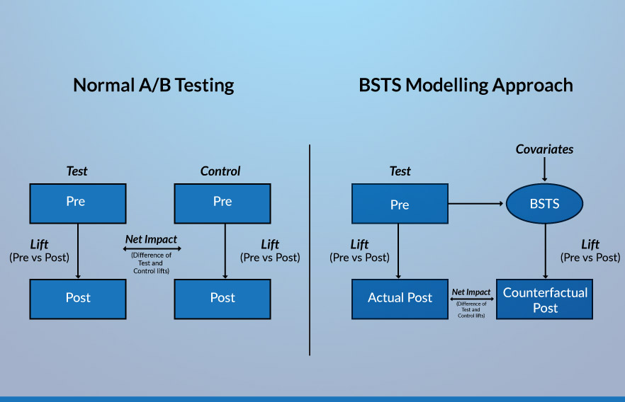
Let us consider a use case of introducing a new channel for searches in a popular browser. Our objective is to calculate its impact on the existing channels in the browser, and on the browser overall, in terms of the number of searches. In this case, since the change was introduced to the entire user population, we do not have a control group to calculate the impact of intervention. Hence, we create a synthetic control group with the same set of users who are part of the test group and then extrapolate the post period values in the absence of an intervention for the relevant attributes.
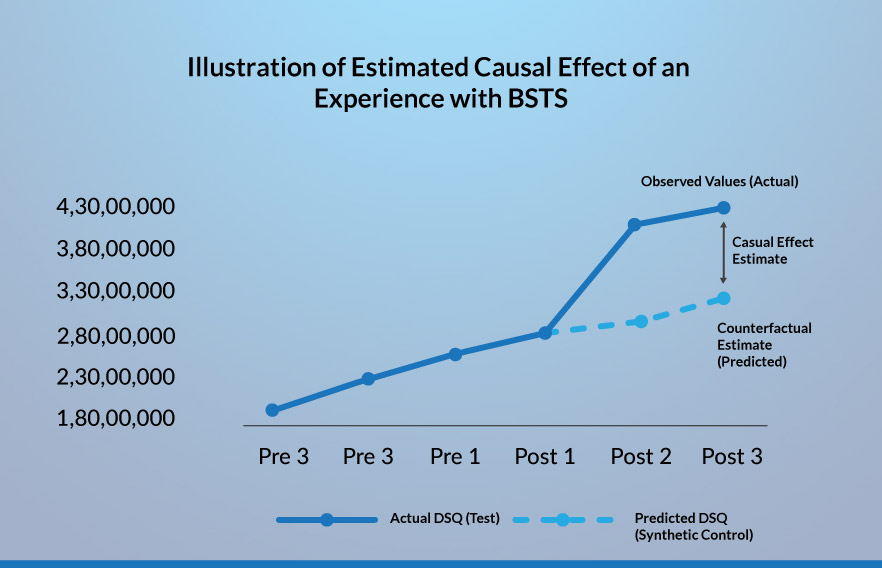
For this process, we use the pre-period numbers of these attributes for the user cohort, and the numbers for a few attributes which are not directly influenced by the intervention to help us in factoring-in the effect of seasonality. The selection of these additional variables is of utmost importance, as if not done properly, could yield unintended results. In this case, we consider the searches made through various channels on other browsers, which we know are not directly influenced by the intervention, for the same timeframe and region. We use these attributes in conjunction with a Bayesian Structural Time Series (BSTS) model to calculate the counterfactual estimates for the user cohort for all the major channels for making searches in the browser.

Impact of the intervention
Now, we also have a control group (albeit, a synthetic control) along with the test group. The difference between the impacts seen by the test group and the control group gives us the causal effect of the intervention. However, in this case, as the pre-period values are the same for both the test and control groups, we directly take the difference between the post period values of these two groups to find the estimated causal impact.

As is the case with conventional A/B testing, we need to check that the difference that we observe is statistically significant. We make use of the p-value for this purpose. Using this, we are able to identify the impact of the intervention on the individual channels for search and on the browser as a whole.
Conclusion
The synthetic control method is extremely useful in cases such as this, where the effect of an intervention needs to be measured in comparison with a scenario in which a control group is not present. However, since a continuous time series data is required to calculate the counterfactual values for the synthetic control group, this won’t be applicable in all cases. In the absence of a continuous time series data, we might have to resort to one of the traditional approaches (or AB testing best practices) to calculate the impact.
Accelerate your Data Engineering capabilities
At LatentView Analytics, we follow a business-focused approach to data in a bid to align analytics and technology. Our workload-centric architectures are designed to meet different data needs of business stakeholders, which come with its own challenges and constraints. To help unleash all levels of data analytics capabilities, realize the full potential of your data and turn it into a competitive advantage for your business, please get in touch with us at marketing@latentview.com


